Ferromagnetism

Abstract

The Ising model is a simplified model of the spin-spin interactions between neighbouring atoms which gives rise to properties of the material such as specific heat capacity and magnetic susceptibility. The Metropolis algorithm is used to model the behaviour of a square array of atoms as the temperature changes.

Introduction

A ferromagnet is a material which exhibits a net magnetic field in the absence of an external magnetic field. The Ising model is used to model the behaviour of ferromagnets and can be used to investigate the behaviour near a phase transition.

↑	↓	↑	↓	↓
↓	↑	↓	↑	↓
↑	↓	↑	↓	↑
↓	↑	↓	↑	↓
↑	↓	↑	↓	↑

Figure 1: Array of atoms with arrows indicating spin direction.

Each atom is signified by a cell in the array and each cell has either spin-up ($+1$) or spin-down ($-1$). By considering these spins we can write an expression for the total interaction energy between the cells. This is given by Equation \eqref{eq:E}

\begin{equation} E = -\frac{1}{2}\sum_{i, j}J_{ij} S_{i}\cdot S_{j} - \mu\sum_{k} S_{k}\cdot B \label{eq:E} \end{equation}

where $J$ is the spin-spin interaction energy per spin squared and $\mu B$ is the external magnetic field interaction energy per spin. The key point to consider here is that when considering the spin-spin interactions, only the interactions between neighbouring cells are considered. So, for a central cells, only the adjacent cells (up, down, left and right) contribute to the total energy and an assumption is made that the other cells do not (i.e. we ignore the interactions from cells that are diagonally located from a given cell.

Method

The Metropolis algorithm used Monte Carlo integration to simulate random selections from a probability density function (PDF). The algorithm is shown in Figure 2. Outside of the algorithm described in Figure 2, there is another to check the state of the system and evaluate whether or not equilibrium has been reached. To determine whether or not equilibrium has been reached, the overall energy of the system is tracked and when the rate of energy change slows down significantly, we can say that the system is approximately at equilibrium.

Once this state has been reached, the Metropolis algorithm is run for another 10,000 and the measurements of $E$ and $S$ are taken from this and later used to calculate $C$ and $\chi$.

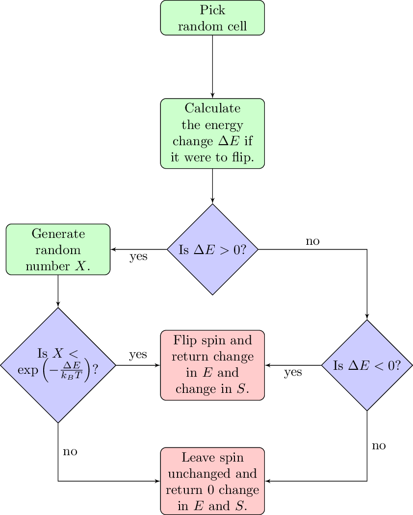
Figure 2: Flow chart describing the implementation of the Metropolis algorithm in this model.

Aside from the Metropolis algorithm, a few other considerations are required. One is for the calculation of the total energy of an array. Considering the first term in Equation \ref{eq:E}, each site has four neighbours. However, if the sum of the four neighbours is taken then there would be some double counting and so to avoid this, we only consider the contribution from the cells to the right and the bottom of the current cell. Therefore, when adding up the cells (and making the array cyclic in $x$ and $y$) we can ensure that every pairwise interaction is accounted for.

Additionally, a substitution is made where $\beta = J/k_{B}T$. This means that the model can be investigated by only varying $\beta$ as opposed to both $J$ and $T$.

To improve the efficiency of the algorithm, the total energy is only calculated once at the start of the simulation. For every subsequent iteration, the energy would be updated by adding or subtracting energy change caused by flipping (or not flipping) a site.

Thermodynamic simulations using the Ising model

Abstract

Introduction

Method

Total energy =

Total energy =

↑	↓	↑	↓	↓
↓	↑	↓	↑	↓
↑	↓	↑	↓	↑
↓	↑	↓	↑	↓
↑	↓	↑	↓	↑

↑	↓	↑	↓	↓
↓	↑	↓	↑	↓
↑	↓	↑	↓	↑
↓	↑	↓	↑	↓
↑	↓	↑	↓	↑

↑	↓	↑	↓	↓
↓	↑	↓	↑	↓
↑	↓	↑	↓	↑
↓	↑	↓	↑	↓
↑	↓	↑	↓	↑